Analysis of Higgs boson decays to four leptons using data and simulation of events at the CMS detector from 2012 using ROOT's RDataFrame

Wunsch, Stefan

Cite as: Wunsch, Stefan; (2021). Analysis of Higgs boson decays to four leptons using data and simulation of events at the CMS detector from 2012 using ROOT's RDataFrame. CERN Open Data Portal. DOI:10.7483/OPENDATA.CMS.F7HD.P3K4

Software Analysis Workflow CMS CERN-LHC

Description

This analysis uses data and simulation of events at the CMS experiment from 2012 with the goal to study decays of a Higgs boson into four leptons, more precisely pairs of electrons or muons. The analysis follows loosely the official CMS analysis published in 2012.

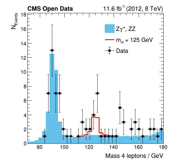
This analysis studies the process $H\rightarrow ZZ\rightarrow 4\ell$, the Higgs boson decaying via two Z bosons into pairs of leptons. We consider here only electrons and muons, which can be directly detected with the CMS detector. The exact same final state is present in events with two Z bosons from quark annihilation, which is the most prominent background process. It should be noted that this analysis takes only this background process into account and neglects the contribution of all other minor background processes. The four leptons can origin from three combinations of lepton pairs: two electron pairs, two muon pairs, or one electron and one muon pair. The analysis is designed to produce the plots in each of these channels but also combines them to a final result, see the example plots below. Further information about the processing steps can be found in the commented source code, the official CMS publication and the similar Open Data analysis using the more complex AOD datasets.

The plot below on the left-hand side shows one of the results of this Open Data analysis, whereas the plot on the right-hand side is taken from the official CMS analysis published in 2012. Both analyses have comparable statistics but the analyzed data is just partially the same. Further, this Open Data analysis neglects for simplicity the minor background processes.

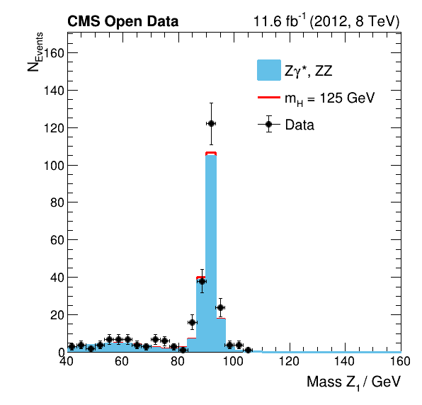
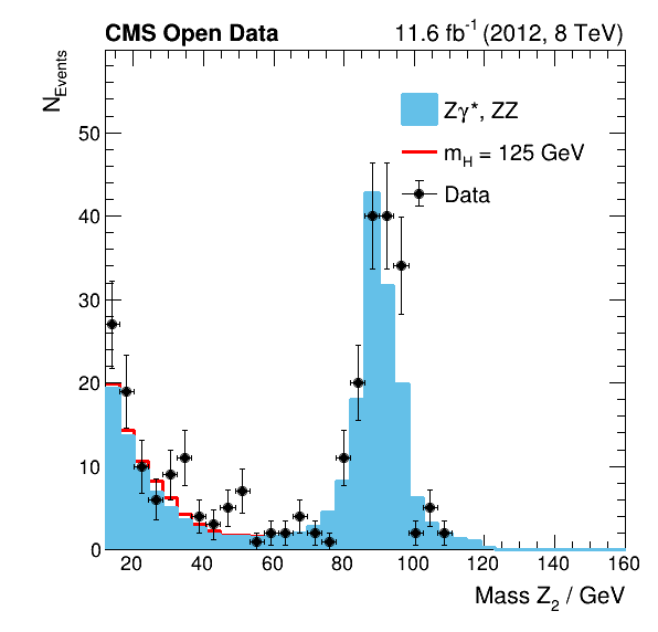
The analysis code of this analysis is designed so that it is easy for you to investigate not just the mass of the Higgs boson but also other features of the data. As an example, the plots below show the reconstructed mass of the two Z bosons, which are the direct decay products of the Higgs boson before those decay again instantly in the analyzed final state particles consisting of electron and muon pairs.

Use with

The analysis can be run with the following datasets:

SMHiggsToZZTo4L dataset in reduced NanoAOD format for education and outreach

ZZTo4mu dataset in reduced NanoAOD format for education and outreach

ZZTo4e dataset in reduced NanoAOD format for education and outreach

ZZTo2e2mu dataset in reduced NanoAOD format for education and outreach

Run2012B_DoubleMuParked dataset in reduced NanoAOD format for education and outreach

Run2012C_DoubleMuParked dataset in reduced NanoAOD format for education and outreach

Run2012B_DoubleElectron dataset in reduced NanoAOD format for education and outreach

Run2012C_DoubleElectron dataset in reduced NanoAOD format for education and outreach

Characteristics

4 files. 290.3 KiB in total.

System details

Software release: ROOT 6.22 or later

How can you use this?

Set up your system with the required software and code

The analysis can be run with a plain ROOT installation, go to root.cern for instructions how to install the software.

In case your system has a CVMFS installation, you can set up the needed software sourcing an LCG software release with the following setup script:

source /cvmfs/sft.cern.ch/lcg/views/LCG_99/x86_64-centos7-gcc10-opt/setup.sh

Note that you may have to replace x86_64-centos7-gcc10-opt with a platform matching your system.

To download the files, you can either use directly the web browser or the following command.

git clone git://github.com/cms-opendata-analyses/HiggsToFourLeptonsNanoAODOutreachAnalysis -b 2012

Step 1: Reduce and pre-process the inital datasets

This step is implemented in the file skim.cxx and is written in C++ for performance reasons. To compile the program, run the following command. Note that you may need to change the compiler based on your system.

g++ -g -O3 -o skim skim.cxx $(root-config --cflags --libs)

The compilation produces a binary, which can be executed as follows.

./skim

The initial datasets are retrieved via network using the XRootD protocol and due to the large size of the dataset the runtime is mainly dependent on your network connection. To speed up multiple executions of the analysis, you can download the files and point to these local copies in the code.

Step 2: Produce histograms

The next step is implemented in Python in the file histograms.py. Run the following command to process the previously produced reduced datasets.

python histograms.py

The script produces the file histograms.root, which contains the histograms. You can have a look at the plain histograms with the ROOT browser opened with the command rootbrowse histograms.root.

Step 3: Combine histograms to plots

To combine the histograms produced in the previous step to meaningful plots, run the following command.

python plot.py

The Python script generates for each variable a png and pdf image file, which can be viewed with a program of your choice. The final plots of the analysis are also included in the source code repository.

Source code repository

https://github.com/cms-opendata-analyses/HiggsToFourLeptonsNanoAODOutreachAnalysis

Disclaimer

GNU General Public License (GPL) version 3